Solving problems in fluid mechanics: The weir problem

I am supervising an intro to fluid dynamics course. My students often find that the maths, formulae and calculations are not difficult, but find it harder to know when to make what assumptions/approximations/simplifications, how to justify them, and then when the formulae apply.

Learning to make appropriate assumptions is probably the most important skill in fluid dynamics, and indeed for applied mathematics in general. Once the right approximations are made, standard results can be applied requiring a series of mostly straightforward calculations.

In this post, we'll go through the weir problem from the second examples sheet, and go step-by-step through each of the assumptions that we make.

The problem states:

Water from a large deep reservoir flows steadily over a long straight weir with a wide crest. Over the weir, the water is of depth $d(x)$ and the free surface has fallen to a level $h(x)$ below that far upstream in the reservoir. Assume that the depth of water varies sufficiently slowly that the velocity is nearly horizontal and uniform in depth, and that $dh/dx$ is non-zero at the crest of the weir. Show that the volume flux (per unit length normal to the flow) is $Q = d \sqrt{2gh}$. From the condition that $Q$ does not vary along the flow, and the condition that $h + d$ is a minimum at the crest of the weir, show that $h = \frac{1}{2} d$ at the crest. Deduce that $Q^2 = 8gL^3/27$ where $L$ is the minimum value of $h + d$.

We are given very little other information: for example, we are not even given a description of the shape of the weir other than that it is long and straight with a wide crest. Nonetheless, this is enough to allow us to make some interesting observations.

Assumptions about water

Let's begin with two background assumptions.

Water is incompressible

The incompressibility assumption asserts that the volume of any given element of fluid remains constant; thus the velocity field $\boldsymbol{u}$ has zero divergence $\nabla \cdot \boldsymbol{u} = 0$. (This results from the conservation of mass equation, $\partial \rho/\partial t + \nabla \cdot (\rho \boldsymbol{u}) = 0$.)

All materials are compressible to some degree or another, but at standard temperatures and pressures, water is close to incompressible, with a bulk modulus of 2.2 GPa (about 10⁴ atmospheres): several orders of magnitude above that of air, and practically infinite in most hydrological applications.

The incompressibility assumption means that volume is conserved: in a steady flow, the volume per unit time that enters a region must equal the volume per unit time that leaves.

Water is inviscid

This assumption is more situational (slippery?).

From the Navier–Stokes equations, we estimate the inertial forces to have approximate magnitude $\rho U^2/ L$ and the viscous forces to have approximate magnitude $\mu U / L^2$; where $\rho$ is the density, $\mu$ is the dynamic viscosity, and $U$ and $L$ are "typical" speeds and lengthscales of the flow. Their ratio defines the Reynolds number $$ \mathrm{Re} = \frac{\rho U^2/L}{\mu U / L^2} = \frac{\rho U L}{\mu} = \frac{UL}{\nu} $$ where $\nu = \mu/\rho$ is the kinematic viscosity.

The value of the Reynolds number depends on the situation at hand. For water, the kinematic viscosity $\nu$ is about $10^{-3} \mathrm{m}^2 \mathrm{s}^{-1}$ (Wikipedia).

In this case, and most other places in this course, it is assumed that the lengthscales and velocity scales are sufficiently large that $\mathrm{Re} \gg 1$, so that the effects of viscosity can be neglected.

The inviscid approximation is useful as it implies that there is no dissipation within the fluid flow. Thus for a steady flow Bernoulli's principle applies, defining a quantity $H$ that is conserved along streamlines.

Viscosity cannot always be neglected. On very small lengthscales and slow speeds, such as $1 \mathrm{mm}$ for a flow at $1 \mathrm{ms}^{-1}$, the Reynolds number is $O(1)$ and so the effects of viscosity are comparable to those of the inertial forces. Even at macroscopic scales, viscosity is responsible for such phenomena as drag on a projectile; a completely inviscid fluid would exert no drag. The limit $\mathrm{Re}\rightarrow\infty$ is said to be a singular limit: the limiting behaviour as $\mathrm{Re}\rightarrow\infty$ is very different from the behaviour at $\mathrm{Re}=\infty$.

The weir problem

For many students – including myself at the time – this was their first time coming across the word weir, so a definition is needed. From Wikipedia:

A weir (/wɪər/), or low-head dam is a barrier across the width of a body of water that alters the flow characteristics of water and usually results in a change in the height of the water level. [...] There are many different types of weirs and they can vary from a simple stone structure that is barely noticeable, to elaborate and very large structures that require extensive management and maintenance.

The weir in this case is a "broad-crested" weir, as opposed to a V-notch weir.

Here's a side view of the weir, labelling the relevant quantities:

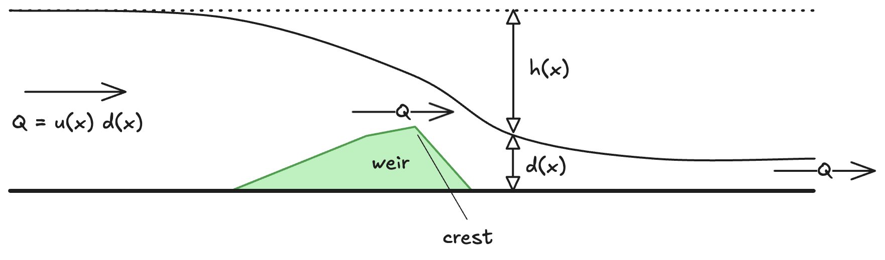
(Sketches by me on Excalidraw.)

Although not specified, it is useful to define two additional quantities. Let $d_U = d(-\infty)$ denote the flow depth far upstream ("a large deep reservoir"), $d_D = d(+\infty)$ be the flow depth far downstream, and let $b(x) = d_U - d(x) - h(x)$ denote the height of the weir. We'll use $y$ to denote the cross-stream direction and $z$ for the depth coordinate relative to the ground far upstream – so $z = d_U - h(x)$ is the position of the free surface.

We shall be evaluating Bernoulli's quantity at the free surface: $$ H = \frac{1}{2}u(x)^2 + g (d_U - h(x)) = \frac{1}{2}u(x)^2 + g (d(x) + b(x)) $$ where the pressure vanishes.

The weir is broad-crested

a wide crest

There are three lengthscales associated with the weir: its length $\mathcal{L}$, its height $\mathcal{H}$ and its width in the cross-stream direction $\mathcal{W}$. The fact that the wave is broad-crested, as opposed to a V-notch, implies that the width is much greater than the length and its height: $\mathcal{W} \gg \mathcal{L} \gg \mathcal{H}$.

While we may speak informally of quantities being "large" or "small", such comparisons should really be made relative to other quantities of the same dimensions.

While it is not specified, we also assume that the channel elsewhere is of a similar width – that the cross-sectional width varies slowly if at all. Thus we may consider the flow to have no component in the cross-stream direction.

Since the channel is wide $\mathcal{W} \gg \mathcal{L}$, variations in the cross-stream direction $y$ are small, since

$$\frac{\partial}{\partial y} \sim \frac{1}{\mathcal{W}} \ll \frac{1}{\mathcal{L}} \sim \frac{\partial}{\partial x}.$$

Thus the flow is assumed to be uniform in $y$. Quantities such as the flow rate can be calculated per unit length:

volume flux (per unit length normal to the flow) is $Q = d \sqrt{2gh}$

Thus $Q$ has units of area flux, $\mathrm{m}^2 \mathrm{s}^{-1}$, not $\mathrm{m}^3 \mathrm{s}^{-1}$.

The weir is long (shallow water approximation)

Assume that the depth of water varies sufficiently slowly...

This is the assumption that $\mathcal{L}\gg\mathcal{H}$, which implies that the gradient of the weir $|db/dx| \sim \mathcal{H}/\mathcal{L} \ll 1$. (Note that the gradient is a nondimensional quantity.)

This is called the shallow water approximation: a flow whose horizontal scales are much greater than its depth. It is extensively used in hydrology; the oceans are "shallow" in this sense.

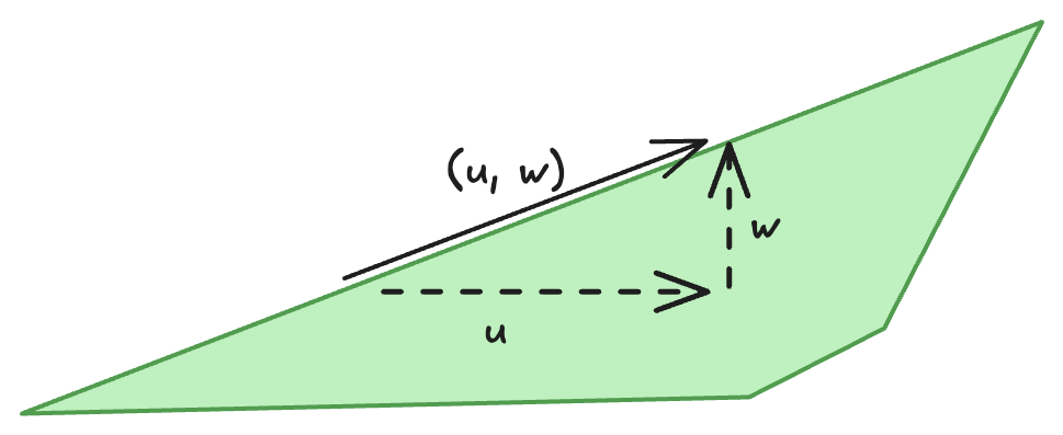
...that the velocity is nearly horizontal...

If $w$ denotes the depthwise component of the velocity, the incompressibility condition implies that $$ \frac{\partial u}{\partial x} + \frac{\partial w}{\partial z} = 0 $$ when we neglect any cross-stream flow. Using the same trick of estimating derivatives as fractions this gives us $$ \frac{u}{\mathcal{L}} \sim \frac{w}{\mathcal{H}} $$ and so $$ \frac{w}{u} = \frac{\mathcal H}{\mathcal L} \ll 1. $$

Another way to see this is by reasoning about the boundary condition at the bottom of the flow. The fact that $b'(x) \ll 1$ implies that the normal to the weir is approximately vertical. The no-penetration condition, which states that the flow must not have any normal component, then implies that the flow is approximately horizontal.

...and uniform in depth.

You might expect that $\mathcal{H}\ll\mathcal{L}$ would imply some shearing in the $z$ direction. However, such a shear profile must arise from internal viscosity, which we are neglecting (as well as assuming that the flow is laminar and not turbulent).

With these assumptions, the velocity field is approximated as $\mathbf{u} = (u(x), 0, 0)$: purely streamwise and with no depthwise or cross-stream dependence. This does in fact violate the condition $\nabla\cdot\mathbf{u} = 0$: the corrections come from the neglected components.

The flow rate per unit length is then $$ Q = \int_{b(x)}^{b(x) + d(x)} u \, dz = d(x)u(x) $$ and this is constant along the flow: $dQ/dx = 0$.¹

The reservoir is deep (subcritical)

large deep reservoir

Since the volume flux $Q = d(x)u(x)$ is independent of $x$, the fact that the upstream depth $d(-\infty) = d_U$ is large implies that the speed $u$ is small, which means the $\frac{1}{2} u^2$ term in Bernoulli's quantity may be neglected.

Again, to say that a dimensional quantity is "large" or "small" requires a comparison against some other quantity. In this case, there are two ways to proceed. The first is to compare the flow depths far upstream and far downstream, asserting that $d_U \gg d_D$: this is a little tricky since in the next section we see that this is not necessarily the case.

Alternatively, we can say that the reservoir is "deep" and the flow is "slow" by comparing the kinetic and potential energy. The total kinetic energy (per unit length) is $$ KE = \int_0^d \frac{1}{2} \rho u^2 \, dz = \frac{1}{2} \rho d u^2, $$ while the total potential energy is $$ GPE = \int_0^d \rho g z \, dz = \frac{1}{2} \rho g d^2. $$ We define the Froude number (Wikipedia) by $$ \mathrm{Fr} = \sqrt\frac{KE}{GPE} = \frac{u}{\sqrt{g d}}. $$

We will say that the reservoir is "deep" if $\mathrm{Fr}\ll 1$. Substituting $Q = du$ gives $$ \mathrm{Fr}^2 = \frac{Q^2}{gd^3}, $$ and so, the assumption is the statement that, far upstream, $$ d^3 \gg \frac{Q^2}{g}, \quad u^3 \ll Qg. $$ In particular, indeed, in Bernoulli's quantity evaluated at the free surface, $$ H = \frac{1}{2} u(x)^2 + g(d_U - h(x)) \approx g d_U $$ since $h(-\infty) = 0$ and $g d_U \gg \frac{1}{2} u^2$.

We say that flows with $\mathrm{Fr} < 1$ are subcritical and flows with $\mathrm{Fr} > 1$ are supercritical. Thus the upstream flow is subcritical.

The flow is steady

We have already been using this assumption by writing everything as functions of $x$, and not of $t$. However, it is important to think about how the steady state is reached.

This in fact depends on the flow conditions far downstream. Specifically, it depends on whether the downstream system can steadily discharge the flow rate $Q$. If the flow rate is increased, or if an obstruction is placed downstream, then the depth of the current must adjust. An obstruction could cause a "traffic jam" to build up and travel backward – a hydraulic jump – until a new equilibrium depth is reached.

These effects are elegantly demonstrated in this video (around the 12:42 mark).

In other words, in a steady state we do not necessarily have a free choice of $d$ and $Q$.

Take another look at the Froude number $\mathrm{Fr} = u/\sqrt{gd}$ and note that $\sqrt{gd}$ is the speed of linear shallow water waves relative to the flow. In the subcritical regime $u < \sqrt{gd}$, waves can travel both upstream and downstream. In some informal sense, waves carry "information"; thus if the flow far downstream is subcritical then "information" about downstream obstacles can travel backwards to influence the flow upstream. This can be formalised using the method of characteristics but requires setting up the shallow water equations (some references).

The flow downstream is supercritical

We have $Q = du$ and $H = \frac{1}{2} u(x)^2 + g(d(x) + b(x)) = gd_U$ as conserved quantities, with the height of the weir $b(x)$ varying along the flow. Substituting out $u$ in the second equation and rearranging gives $$ \frac{Q^2}{2d(x)^2} + g d(x) = g (d_U - b(x)) $$ Thus at a given position $x$ there is a certain value of $b(x)$ and this relation determines $d(x)$.

The following graph shows the expression on the left $Q^2/(2d^2) + g d$ as a function of $d$ in red, in units in which $Q = 1$ and $g = 1$.

(thanks Desmos)

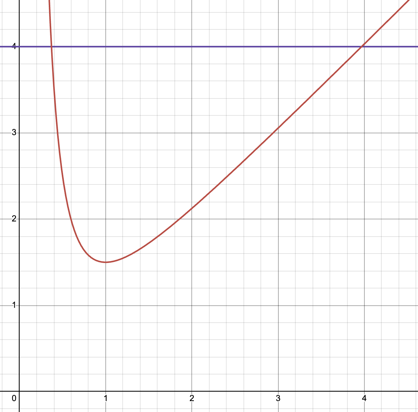
A little algebra shows that the minimum occurs at $d = (Q^2/g)^{1/3}$ (which is $d=1$ in these units), and that the minimum value is $3/2$.

The right hand expression $g(d_U - b(x))$ does not depend on $d$, so it is a horizontal line, that slides down as $b$ is increased and then slides back up as $b$ decreases. For any given value of $b$, provided it is not too large, there are two solutions for $d$: one with $d > (Q^2/g)^{1/3}$ and one with $d < (Q^2/g)^{1/3}$. These correspond to subcritical and supercritical flow regimes respectively.

We know that the flow far upstream is subcritical, which means we must be starting with the branch on the right. As $b$ increases, the blue line goes down and so $d$ decreases, but initially stays on the branch on the right.

Assume [...] that $dh/dx$ is non-zero at the crest of the weir

At the crest $b$ reaches its maximum. As $b$ decreases again, the blue line moves back up but $d$ is not going back up; which means we must be switching to the left branch. Thus $b$ reached its maximum value when $d = (Q^2 / g)^{1/3}$, making the transition between a supercritical and a subcritical flow. The downstream flow is supercritical, taking the other branch.

Conclusion

I'm quite fond of this problem because it's a good introduction to many standard assumptions that one makes when modelling fluid flows.

We started with the usual assumptions about water flows (in this course):

• Incompressible gives us conservation of volume.
• Inviscid means we can use Bernoulli's principle as there is no loss.

Then we made some assumptions about the flow geometry:

• Shallow geometry $\mathcal{L} \gg \mathcal{H}$ means the flow is approximately horizontal; and so the flow rate is just $Q = du$.
• Wide geometry $\mathcal{W} \gg \mathcal{L}$ means the flow can be assumed to be uniform across the channel.
• Steady means no time derivatives – but raises the question of how one arrived at the steady state.

Finally we used some facts that were more specific to this problem:

• The upstream reservoir is deep, which means the potential energy is much greater than the kinetic energy, which simplifies the Bernoulli quantity $H$.
• The flow downstream is supercritical, so it can have a different depth from the upstream flow while maintaining conservation of $Q$ and $H$.

With practice, one learns to spot other similar situations in which these approximations may be used, and situations where they may not.

---

1. To show this, differentiate under the integral sign and take care with the boundary conditions at $z=b$ and $z=b+d$. ↩