The semitone filter: Adding a pipe organ to The Magic Flute Overture

Over the Christmas holiday I've had a chance to play around with a few ideas that I've had with signal processing. One idea that I had was to try a "semitone filter", emphasising out precisely certain frequencies in an audio signal while suppressing all others.

This is not the same thing as Auto-Tune, but it has a similar effect of producing a sound that is brighter and more harmonic, and the result sounds something like a pipe organ.

In the demonstration that follows I shall run this filter on this recording of the Overture from The Magic Flute, which I have downloaded as original.ogg.

Loading the file and basic properties

We shall use the soundfile library, which takes care of the nitty-gritty business of reading different file formats.

starttime = 76
endtime = 194

# alternatively:
# starttime = 0
# endtime = None

with open('original.ogg', 'rb') as origf:
    fd = soundfile.SoundFile(origf)
    sr = fd.samplerate  # 44100 Hz
    if starttime:
        fd.seek(starttime * sr)
    if endtime is not None:
        multichan_sig = fd.read(sr * (endtime - starttime))
    else:
        multichan_sig = fd.read()

# Collapse it to a single channel
sig = np.mean(multichan_sig, axis=1)

# Calculate the Fourier transform
sigfft = np.fft.rfft(sig)

Here's what this excerpt sounds like:

Define the time and frequency domains

ts = np.arange(sig.shape[0]) / sr  
# 17,816,400 samples for the full file
# 5,203,800 for the trimmed file
freqs = np.fft.rfftfreq(n=ts.shape[0], d=1/sr)  
# half as many

Note that since sig is a real-valued signal, we can use the rfft, irfft, rfftfreq, etc. functions in np.fft, since we only need the positive values in the frequency domain to eventually recover a real signal. Thus the frequency domain is half the size of the time domain (plus one for the f = 0 mode).

Creating and applying the filter

Overview

The transfer function (frequency response) of this filter will look something like this:

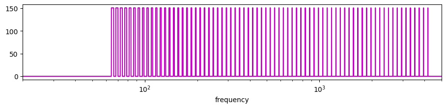
That is, it shall pick out frequency components that are very close to the pitch in the chromatic scale, while elminating all other frequency components. Essentially it is a combination of many band-pass filters. It is similar to the comb filter except that the responses are not spaced apart uniformly, but logarithmically.¹

The idea is that we multiply the Fourier transform of our signal by the transfer function in order to apply the signal. Unlike something like Auto-Tune, we are not adjusting any frequency components that are off-key; we are simply eliminating them. So, a sine tone that is in between two semitones will be reduced or eliminated, rather than being adjusted to the nearest semitone.

Start by defining the pitches of the chromatic scale:

# Number of semitones relative to A440
steps = np.arange(-33, 40, 1) # C2 to C8
pitches = 440 * 2 ** (steps / 12)

print(np.min(pitches))  # np.float64(65.40639132514966)
print(np.max(pitches))  # np.float64(4186.009044809578)

It is possible to take other combinations of frequencies, including inharmonic combinations. But for this discussion we take the chromatic scale, so that we can bring out concordance and suppress discordance.

The undamped filter

There are several options for defining the filter. One is to use "top-hat functions" (step functions); alternatively each of these "needles" could be a very narrow Gaussian, which will keep some amount of the intermediate frequency components. This choice doesn't make much difference in the end result, although an important parameter that we will consider is the "tolerance" or width of each needle.

# Width of each needle
tol = 1  # Hz

undampened_transfer = np.zeros_like(freqs)

for pitch in pitches:
    # Gaussian
    # undampened_transfer += np.exp(-((freqs - pitch)/tol)**2)
    
    # top-hat
    mask = (np.abs(freqs - pitch) < tol)
    undampened_transfer[mask] += 1

# Normalization (so that the volume is the same)
undampened_transfer /= np.mean(undampened_transfer)

A note the use of the for loop here: while for loops in Python are typically much slower than equivalents provided by numpy, in this example the pitches array consists of only about 100 entries, and so it is not really necessary to optimise this. My original attempt at this had used something like np.meshgrid to create meshes of the freqs and pitches arrays; while this would allow us to use numpy methods and avoid the for loop, it would have increased the memory footprint by 200 times! This is unacceptable for an array as large as freqs.

Now apply the filter to the signal:

undampened_filtered = np.fft.irfft(sigfft * undampened_transfer)

# normalise to avoid clipping
undampened_filtered /= np.max(np.abs(undampened_filtered))

# Save the file as an MP3
soundfile.write(
    "undampened_filtered.mp3", undampened_filtered,
    samplerate=sr,
    format="MP3",
    subtype="MPEG_LAYER_III",
)

# Display it (in a Jupyter notebook)
display.Audio(undampened_filtered, rate=sr)

giving rise to:

Applying dampening

This sounds rather dreadful. Although faint traces of the original can be heard, it is hidden behind a mush that sounds like a cat sitting on an organ keyboard.

This is because the Fourier transform is a global operation: each frequency component in the FFT uses information from the entire signal. And consequently, when the filter is applied and the IFFT is computed, each part of the signal is affected by every other part of the signal. Loud bits don't remain loud, quiet bits don't remain quiet, and any components from elsewhere are picked up. That A at the end gets mushed in with the E flat at the beginning.

That said, the timbre does sound very bright, indeed like an organ: this is because we have filtered out all inharmonicities, leaving only tones that correspond to exact semitone values, whose frequencies are integer multiples of each other (ok, up to equal temperament). It's just a shame that we are picking up tones from everywhere else in the piece.

There are different options for dealing with the nonlocality. One way is to use a short-time Fourier transform instead of the full FFT. A much simpler method is to apply a dampening to the filter.

First, we recover the kernel of this undampened filter by inverting the Fourier transform:

undampened_filt = np.fft.irfft(undampened_transfer)

By the convolution theorem, our multiplicative filter was equivalent to convolution of our signal with this kernel.

Let's multiply our kernel by an exponentially decaying function (in the time domain), so that the signal is affected only by nearby times. Then compute the FFT for this dampened kernel to retrieve the new transfer function.

# Sustain time; a higher value creates a "mushier" sound
sustain = 10 # seconds

# get rid of nonlocal effects
# otherwise it's a forever damper pedal
filt = undampened_filt * np.exp(-ts/sustain)

transfer = np.fft.rfft(filt)
transfer /= np.mean(transfer) # normalization

The dampened transfer function as a function of frequency is plotted below. In the top diagram, we see the real and imaginary parts of this function. The bottom diagram compares the magnitudes of the undampened (black) and dampened (red) transfer functions.

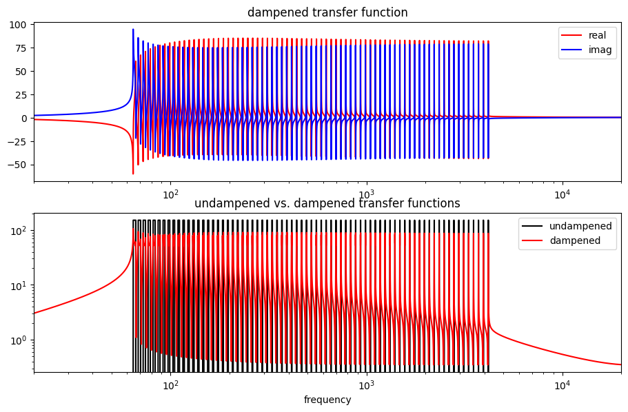
Unlike the undampened version, the dampened version (a) has a nonzero imaginary part (i.e. nonconstant phase) and (b) has components at very low and very high frequencies, both of which will contribute to the requirement of correcting and eliminating nonlocal effects.

When we apply this dampened filter, we get a very different sound.

filtered = np.fft.irfft(sigfft * transfer)
soundfile.write(
    "filtered.mp3", filtered,
    samplerate=sr,
    format="MP3",
    subtype="MPEG_LAYER_III",
)

Conclusion

I think this sounds rather pleasant (at least in parts): as though a pipe organ had been added to the orchestration, and it were being performed in a large and reverberant room. The overall shape, dynamics and harmony of the original are preserved, but there are a shimmer and an etherealness to the sound. The very low frequencies and short-attack hits of the timpani are still markedly audible.

Here's the full Overture with the filter applied.

There's still some sound at the beginning of the track before the first note is played, because we haven't completely eliminated nonlocal effects. I can't tell whether the filter is "the right way round" – whether echoes and reverberations are happening after the note or before. The dampening that we applied had a characteristic timescale of 10 seconds – quite a long reverb time, and at times long enough that notes from one bar are "bleeding over" into the next bar.

Perhaps a shorter time would have been appropriate, although I imagine it depends on the "harmonic tempo" of the piece, how often chord changes happen, etc.: this piece has quite a slow harmonic tempo and mostly goes between the tonic and dominant, which share many of the same concordant tones, so the bleeding isn't as awful as I would have thought. The worst sound is a couple of bars from the end, when chords alternate between the tonic and the dominant very quickly.

Another interesting observation is that the distortion seems to selectively affect the strings, while the wind and timpani sounds are more or less unaffected. My guess is that the flutes produce very harmonic sounds anyway, so this filter doesn't really affect them, while the timpani has a range of both low and high frequency components and so most of its sound is captured.²

Anyway, this was just something I was playing around with over my Christmas break. I had a few other ideas too, which I shall write up in due course. I probably won't be using it for any orchestra or concert band recordings (God forbid choir), although it's an interesting effect that is possibly useful if you want to add a sparkle to the sound of your track without greatly distorting the frequencies.

1. A previous version of this post erroneously claimed that this is "dual" to the comb filter, confusing the frequency response with the impulse response. ↩
2. Although the pitches of the timp notes are very low, the actual spectrum is very broad because of the short percussive nature of the sound, bringing high frequency components. ↩